
Introduction:
The past two decades have seen the development and application of numerous quantitative approaches in the geosciences. Ranging from spectral to cluster analysis, these approaches have found wide application throughout geosciences and have been used for process simulation, modelling, mapping, stratigraphic analysis and correlation, classification and prediction. Most of the quantitative approaches applied in the past two decades have been statistical in nature. Their application has permitted systematic, rapid and objective analysis and processing of geological data. The usefulness of any of these methods depends in large part on the nature of the problem to be solved as they often
try to simplify processes that are acting in a complicated, dynamic and often nonlinear way. Artificial intelligence broadly defines such computing techniques as expert systems, fuzzy set logic and computer neural networks (CNN). These have been developed as a result of the cooperative efforts made by scientists from many disciplines such as mathematics (traditional statistics), computer science, biology and psychology. Among these approaches, CNN’s are the most appealing to geologists.

The types of problems that lend themselves to a CNN approach are:
(I) where the problem area is rich in historical data or examples;
(2) where data are numeric and are intrinsically noisy;
(3) where the discriminator or function to determine solutions is unknown or expensive to discover;
(4) where the problem is dependent upon multiple interacting parameters whose interdependence is too realistically difficult to describe; and
(5) where conventional approaches are inadequate because the problem is too complex for a programmer to find procedural solutions.
THE ALGORITHM AND NEURAL NETWOK IMPIEMNTATION:
The CRNN algorithm has little resemblance to the more widely used BP-CNN but it is similar to the probabilistic neural network (Specht, 1990). No iteration is involved in computing with the GRNN algorithm. It has, at its root, one of the most commonly used statistical techniques – regression analysis. To perform regression, one has to assume (or guess) a certain functional form to analyze the data points and to determine the parameters of the function. The limitation of this approach is in the choice of the function. If the wrong functional form is assumed, the value of the established function for prediction is reduced. The GRNN algorithm proposed by Sprcht (1991) successfully overcomes this shortcoming by not requiring an assumption in the form of the regression function. Instead, it approaches the problem on the basis of the probability density function of the observed data (or the training examples). Thus, there is no need to determine parameters for the function. Another attractive feature is that, unlike BP-CNNs, a GRNN does not converge to local minima (Specht, 1991). Also, the training process with a GRNN-type algorithm is much more efficient than with the BP-CNN algorithm (Specht and Shepiro, I 990). Mathematically, general regression obtains the conditional mean of y. a scalar random variable v, when given X (a particular measured value of a vector random variable x) using nonparametric estimator of the joint probability density function f(x. y). In the algorithm Specht (1991) employs a class of consistent estimators proposed by Parzen (1962) for this purpose. These estimators are based upon sample values Xi and Y, and are proven to be also applicable to the multidimensional case 1966). With different estimators,2 forms of general regression are proposed.
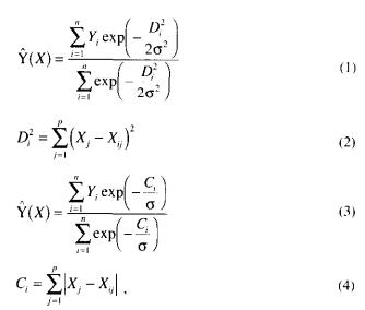
where n is number of sample values Xi and Yi , Di^2 is the Euclidean distance between X and Xi with vector size p, while Ci is their city block distance and sigma is a smoothing factor. From equations (I) and (3) we can see that general regression is actually a weighted average of all of the observed values. Yi, where each observed value is weighted exponentially according to its Euclidean or city block distance tom X. When the smoothing factor sigma becomes very large, Y(X)-cap becomes the mean of the observed Yi. When sigma approaches zero, Y(X)-cap assumes the value of the Yi associated with the Xi which approaches x. With intermediate values of sigma, all values of k; contribute to Y(X)-cap. With those corresponding to points closer to X being given heavier weight. In general regression, sigma is the only important computing parameter to be determined. When n is very large, for efficiency of general regression it is necessary to group the observations into a smaller number of clusters. Many clustering techniques can he used. The cluster version of general regression can he written as:
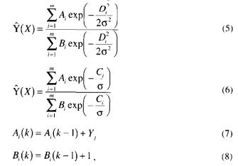
Where m is the number of the cluster. Ai and Bi, are the value of the coefficients for cluster i after k observations. Ai is actually the sum of the Y values and Bi the number of observations grouped into cluster i. Those coefficients can be determined in one pass through the observed samples. A very simple clustering method is to set a single radius, r, with certain information from the data set. The first date point is arbitrarily taken as the first cluster centre. If the second data point has a distance from this cluster centre less than I, the first cluster centre is updated with equations (7) and (8); otherwise, the second data point becomes a new (second) cluster centre. Each future data point from the data set is processed in this way.
In terms of computer neural network technique, a GRNN constructed on the basis of equations (5), (7) and (8) or (6), (7) and (8) consists of four layers (Figure I). The input layer provides all of the scaled input variables (X) and is fully connected to the pattern layer. The weights of each pattern unit that connect to the input layer actually represent a cluster centre in a multidimensional space. The A and B coefficients associated with these clusters serve as the weights connecting the pattern layer and the summation layer. The unit(s) in output layer receive results from the summation units and then calculate the output.
Major attractions of the GRNN algorithm are that it will not converge to a local minimum (Specht, 1991) and, furthermore, it is not necessary to determine the network architecture. The single important parameter. Sigma, can be automatically determined during training. In addition. GRNNs need fewer examples then BP-CNNs to be properly trained. Therefore, GRNNs are an attractive and promising alternative to BP-CNNs for use in geosciences. The following two examples illustrate the usefulness of GRNN. Further explanation is warranted on how the radius of influence is determined. The program first calculates all of the distances among the data points in the training set and finds the difference between the maximum and minimum inter data distance. If the training data set is small (N< 50), the minimum distance plus 5% of the difference is taken 8s the radius of influence for
clustering; if the training data set is large (N > 50), the minimum distance plus 10% of the difference is taken as the radius. We also experimented with different types of distance (Euclidean versus city block). In the later discussion, the use of equation (5) in training and testing is referred to as mode I and the use of equation (6) as mode 2.
For application examples refer to: Canadian Journal of exploration geophysicists (vol-30)
